In the realm of probability and statistics, understanding the types of probability distributions is crucial. Two primary types of distributions are discrete and continuous probability distributions. Both play significant roles in various fields, from finance to engineering, and even in everyday decision-making. This article delves into the differences between discrete and continuous probability distributions, their uses, and how they are applied in real-world scenarios.

What are Probability Distributions?

Probability distributions describe how the values of a random variable are distributed. They provide a comprehensive view of the likelihood of different outcomes. Probability distributions can be broadly categorized into discrete and continuous distributions.

Discrete Probability Distributions

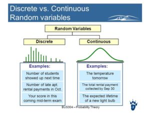
Discrete probability distributions apply to scenarios where the set of possible outcomes is countable and finite. These distributions are characterized by distinct, separate values. Common examples include rolling a die, flipping a coin, or the number of students in a classroom.

Key Features of Discrete Distributions

1. Countable Outcomes: The possible outcomes can be listed out, such as {1, 2, 3, 4, 5, 6} for a die roll.
2. Probability Mass Function (PMF): This function assigns probabilities to each possible outcome. The sum of all probabilities in a discrete distribution equals 1.
3. Examples:
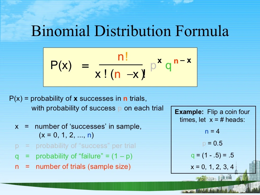
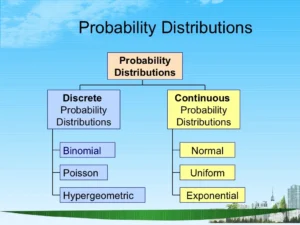
   • Binomial Distribution: Describes the number of successes in a fixed number of independent Bernoulli trials (e.g., flipping a coin multiple times).
   • Poisson Distribution: Models the number of events occurring within a fixed interval of time or space (e.g., the number of emails received in an hour).

Uses of Discrete Distributions

• Quality Control: Determining the number of defective items in a batch.
• Risk Assessment: Evaluating the likelihood of different risk scenarios.
• Inventory Management: Predicting the number of units sold in a day.

Continuous Probability Distributions

Continuous probability distributions, on the other hand, apply to scenarios where the set of possible outcomes is uncountable and infinite. These distributions are characterized by a continuous range of values. Examples include measuring time, temperature, or the height of individuals.

Key Features of Continuous Distributions

1. Uncountable Outcomes: The possible outcomes form a continuum, such as all real numbers between 0 and 1.
2. Probability Density Function (PDF): Instead of assigning probabilities to specific outcomes, a PDF describes the likelihood of the variable falling within a particular range.
3. Examples:
   • Normal Distribution: Also known as the Gaussian distribution, it is symmetrical and describes many natural phenomena (e.g., heights of people).
   • Exponential Distribution: Models the time between events in a Poisson process (e.g., the time between arrivals of buses).

Uses of Continuous Distributions

• Natural Sciences: Modeling phenomena like temperature changes or biological measurements.
• Finance: Analyzing stock prices and returns, which are often assumed to be normally distributed.
• Engineering: Assessing time-to-failure of mechanical systems.

Differences Between Discrete

1. Nature of Outcomes: Discrete distributions deal with countable outcomes, while continuous distributions handle uncountable outcomes.
2. Function Type: Discrete distributions use a Probability Mass Function (PMF), whereas continuous distributions use a Probability Density Function (PDF).
3. Cumulative Distribution Function (CDF): Both types use a CDF to describe the probability that a random variable will take a value less than or equal to a given point. However, the integration for continuous distributions involves calculus due to the nature of the PDF.
4. Applications: Discrete distributions are often used in quality control, inventory management, and risk assessment, while continuous distributions are prevalent in natural sciences, finance, and engineering.

Real-World Applications

Healthcare

• Discrete: Modeling the number of patients arriving at a clinic in a day (Poisson distribution).
• Continuous: Measuring the time until a patient recovers from surgery (Exponential distribution).

Finance

• Discrete: Counting the number of stock trades in a day.
• Continuous: Analyzing the distribution of returns on an investment portfolio.

Engineering

• Discrete: Assessing the number of defective parts in a manufacturing process.
• Continuous: Evaluating the lifespan of a lightbulb using a Weibull distribution.

Conclusion

Understanding the differences between discrete and continuous probability distributions is fundamental for applying statistical methods correctly. Discrete distributions are suitable for countable outcomes and scenarios involving distinct values, while continuous distributions apply to measurements and scenarios with an infinite range of possible outcomes. By recognizing the appropriate distribution type, professionals across various fields can make more informed decisions, ensuring accurate data analysis and effective problem-solving.