Unlocking the Variability in Data: The Power of Dispersion Measures

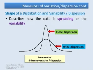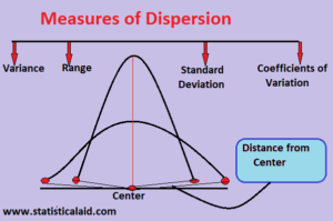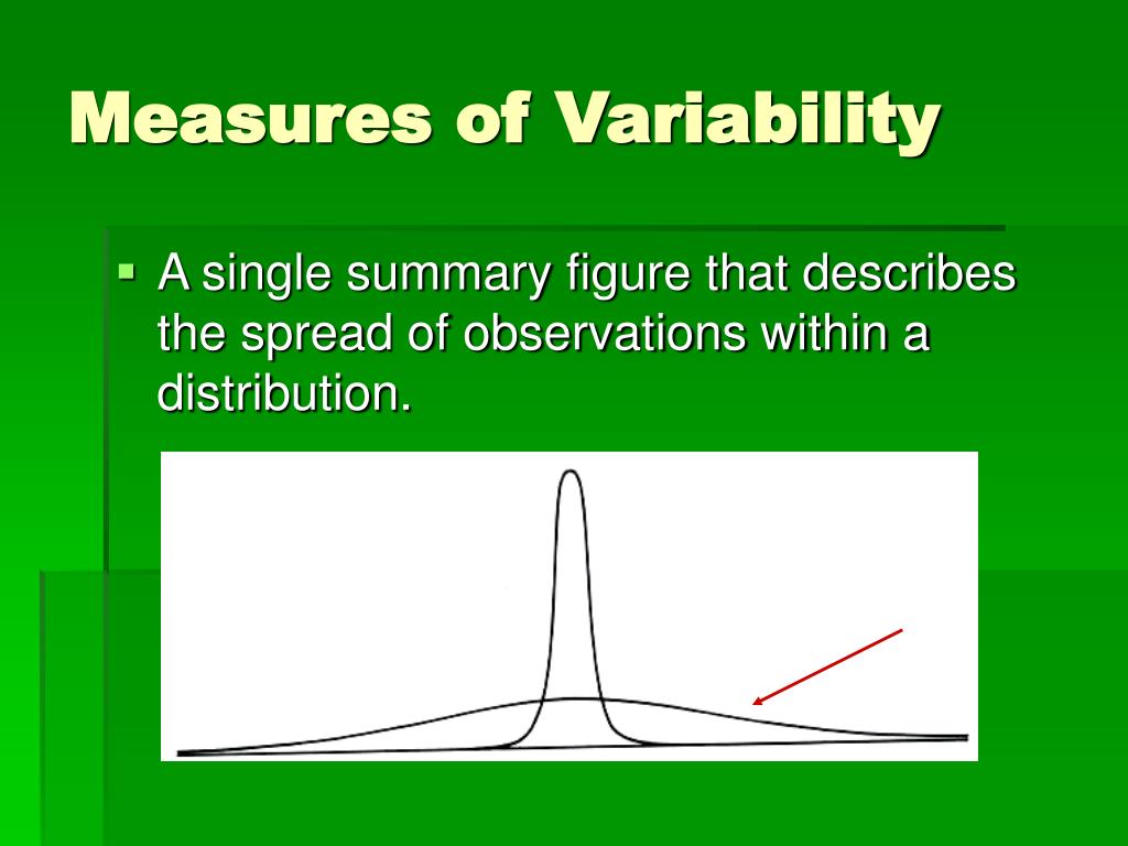
Understanding data variability is crucial in a world driven by data. Dispersion measures offer insights into the spread of data points in a dataset, revealing how much individual data values differ from the average. This understanding can significantly impact decision-making across various fields, from business and finance to healthcare and scientific research. This article explores the power of dispersion measures, detailing how they can unlock valuable insights and improve data analysis.

What Are Dispersion Measures?

Dispersion measures, also known as measures of variability or spread, describe the extent to which data points in a dataset deviate from the mean. Unlike central tendency measures (mean, median, mode), which provide information about the center of the data, dispersion measures offer insights into the variability within the dataset. Common dispersion measures include range, variance, standard deviation, and interquartile range (IQR).

Why Are Dispersion Measures Important?

1. Understanding Data Spread: Dispersion measures help to understand how data points are distributed around the central value. This understanding is crucial for assessing the reliability and consistency of data.
2. Comparing Datasets: They allow comparisons between different datasets. For instance, comparing the standard deviation of exam scores across different classes can reveal which class has more consistent performance.
3. Risk Assessment: In finance, dispersion measures like standard deviation are used to assess the risk associated with investment portfolios. A higher standard deviation indicates higher risk.
4. Improving Predictions: Accurate predictions require understanding the variability in data. Measures of dispersion can help in refining predictive models by accounting for data spread.

Common Dispersion Measures

1. Range

The range is the simplest measure of dispersion. It is calculated by subtracting the smallest value from the largest value in the dataset.

Formula: $\text{Range}=\text{Maximum Value}-\text{Minimum Value}$

Example: In a dataset of exam scores: 55, 65, 70, 80, and 90, the range is: $90-55=35$

Pros:

• Easy to calculate.
• Provides a quick sense of the data spread.

Cons:

• Sensitive to outliers.
• Doesn’t account for the distribution of all values.

2. Variance

Variance measures the average squared deviation of each data point from the mean. It provides a more comprehensive view of data spread than the range.

Formula: Variance=∑(xi−μ)2N\text{Variance} = \frac{\sum (x_i – \mu)^2}{N}Variance=N∑(xi​−μ)2​ where xix_ixi​ represents each data point, $\mu$ is the mean of the data, and $N$ is the number of data points.

Example: For the dataset: 55, 65, 70, 80, and 90:

1. Calculate the mean: μ=55+65+70+80+905=72\mu = \frac{55 + 65 + 70 + 80 + 90}{5} = 72μ=555+65+70+80+90​=72
2. Compute the squared deviations and their average.

Pros:

• Takes into account all data points.
• Provides a measure of data dispersion in squared units.

Cons:

• The units of variance are not the same as the original data, making it less intuitive.

3. Standard Deviation

The standard deviation is the square root of the variance and provides a measure of dispersion in the same units as the data.

Formula: Standard Deviation=Variance\text{Standard Deviation} = \sqrt{\text{Variance}}Standard Deviation=Variance​

Example: For the same dataset:

1. Compute the variance.
2. Take the square root of the variance.

Pros:

• Easier to interpret than variance.
• Expresses dispersion in the same units as the data.

Cons:

• Like variance, it is sensitive to outliers.

4. Interquartile Range (IQR)

The IQR measures the range within which the central 50% of the data lies, effectively removing the influence of outliers.

Formula: $\text{IQR}=Q3-Q1$ where $Q3$ is the third quartile and $Q1$ is the first quartile.

Example: For a dataset: 55, 65, 70, 80, and 90:

1. Sort the data and find $Q1$ and $Q3$.
2. Compute the IQR.

Pros:

• Less sensitive to outliers.
• Provides a clear picture of the middle spread of the data.

Cons:

• Does not account for the variability in the extremes of the dataset.

Applications of Dispersion Measures

1. Business Analytics: Companies use dispersion measures to analyze sales performance, customer satisfaction, and market trends. Understanding variability helps in optimizing operations and predicting future trends.
2. Healthcare: In clinical trials, dispersion measures are used to assess the effectiveness and safety of treatments by analyzing the variability in patient responses.
3. Education: Educators use dispersion measures to evaluate the consistency of student performance and the effectiveness of teaching methods.
4. Finance: Investors use measures like standard deviation to assess the risk associated with different investments and to build diversified portfolios.

Choosing the Right Dispersion Measure

Selecting the appropriate dispersion measure depends on the context and goals of the analysis. For datasets with significant outliers, the IQR might be more suitable, while variance and standard deviation are useful for datasets where the mean is a good representation of central tendency.

Conclusion

Dispersion measures are powerful tools for understanding data variability and making informed decisions based on data analysis. By leveraging range, variance, standard deviation, and interquartile range, individuals and organizations can gain deeper insights into their data, leading to better predictions, risk assessments, and strategic decisions. Embracing these measures enhances the ability to interpret data comprehensively and apply findings effectively in various fields.