Mastering Measures of Dispersion: A Comprehensive Guide for Data Scientists in 2024

In the world of data science, understanding how data varies is crucial for making informed decisions and drawing accurate conclusions. Measures of dispersion, also known as measures of variability, provide insights into the spread and variability of data points within a dataset. This comprehensive guide will explore key measures of dispersion, their significance, and how data scientists can effectively use them in 2024.

What Are Measures of Dispersion?

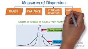
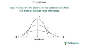
Measures of dispersion quantify the extent to which data points in a dataset differ from the mean or central value. Unlike measures of central tendency (such as mean, median, and mode), which provide information about the center of a data distribution, measures of dispersion reveal how spread out the data points are. This information is vital for understanding the distribution and variability of data, which can impact statistical analyses and decision-making processes.

Key Measures of Dispersion

1. Range

   The range is the simplest measure of dispersion. It is calculated by subtracting the minimum value from the maximum value in a dataset.

   Formula:

   $$\text{Range}=\text{Maximum Value}-\text{Minimum Value}$$Example: For a dataset with values [3, 7, 5, 9, 12], the range is $12-3=9$.

   Pros and Cons:

   • Pros: Easy to calculate and understand.
   • Cons: Sensitive to outliers and does not provide information about the distribution of values between the extremes.
2. Variance

   Variance measures the average squared deviation of each data point from the mean. It provides an indication of how spread out the data points are around the mean.

   Formula:

   Variance(σ2)=1N∑i=1N(xi−xˉ)2\text{Variance} (\sigma^2) = \frac{1}{N} \sum_{i=1}^{N} (x_i – \bar{x})^2Variance(σ2)=N1​i=1∑N​(xi​−xˉ)2Where xix_ixi​ represents each data point, xˉ\bar{x}xˉ is the mean of the dataset, and $N$ is the number of data points.

   Example: For a dataset [4, 8, 6, 5], the mean is 5.75. The variance is calculated as follows:

   Variance=(4−5.75)2+(8−5.75)2+(6−5.75)2+(5−5.75)24\text{Variance} = \frac{(4 – 5.75)^2 + (8 – 5.75)^2 + (6 – 5.75)^2 + (5 – 5.75)^2}{4}Variance=4(4−5.75)2+(8−5.75)2+(6−5.75)2+(5−5.75)2​ Variance=(3.06+5.06+0.06+0.56)4=2.44\text{Variance} = \frac{(3.06 + 5.06 + 0.06 + 0.56)}{4} = 2.44Variance=4(3.06+5.06+0.06+0.56)​=2.44Pros and Cons:

   • Pros: Provides a detailed measure of dispersion and is fundamental in statistical analysis.
   • Cons: The squared units can make interpretation less intuitive.
3. Standard Deviation

   Standard deviation is the square root of the variance. It represents the average distance of data points from the mean in the same units as the original data.

   Formula:

   Standard Deviation(σ)=Variance\text{Standard Deviation} (\sigma) = \sqrt{\text{Variance}}Standard Deviation(σ)=Variance​Example: Continuing from the previous variance example, the standard deviation is:

   Standard Deviation=2.44≈1.56\text{Standard Deviation} = \sqrt{2.44} \approx 1.56Standard Deviation=2.44​≈1.56Pros and Cons:

   • Pros: Provides a clear measure of dispersion in the same units as the data, making it easier to interpret.
   • Cons: Like variance, it is affected by outliers.
4. Interquartile Range (IQR)

   The interquartile range measures the spread of the middle 50% of data points. It is calculated by subtracting the first quartile (Q1) from the third quartile (Q3).

   Formula:

   $$\text{IQR}=Q3-Q1$$Example: For a dataset arranged in ascending order [2, 4, 6, 8, 10, 12, 14], Q1 is 4, and Q3 is 10. Thus, the IQR is $10-4=6$.

   Pros and Cons:

   • Pros: Less sensitive to outliers and provides a clear view of the central spread.
   • Cons: Does not account for variability outside the middle 50% of the data.
5. Coefficient of Variation (CV)

   The coefficient of variation is a normalized measure of dispersion that expresses the standard deviation as a percentage of the mean. It is useful for comparing variability between datasets with different units or scales.

   Formula:

   CV=(Standard DeviationMean)×100%\text{CV} = \left( \frac{\text{Standard Deviation}}{\text{Mean}} \right) \times 100\%CV=(MeanStandard Deviation​)×100%Example: If a dataset has a mean of 20 and a standard deviation of 4, the CV is:

   CV=(420)×100%=20%\text{CV} = \left( \frac{4}{20} \right) \times 100\% = 20\%CV=(204​)×100%=20%Pros and Cons:

   • Pros: Useful for comparing variability across different datasets or variables.
   • Cons: Less informative if the mean is very close to zero.

Applications of Measures of Dispersion in Data Science

Understanding measures of dispersion is critical for various data science tasks, including:

1. Data Preprocessing: Identifying and handling outliers. For example, a high range or standard deviation might indicate the presence of outliers that need to be addressed.
2. Statistical Analysis: Conducting hypothesis tests and building confidence intervals. Measures of dispersion help in assessing the reliability of statistical estimates.
3. Model Evaluation: Comparing the performance of different models. Variability in predictions can reveal how consistently a model performs.
4. Risk Management: In finance and investment, measures of dispersion are used to assess the risk associated with different assets or portfolios.

Best Practices for Using Measures of Dispersion

1. Choose the Right Measure: Different measures provide different insights. For example, use the IQR when you need to understand the spread of the central data points and the standard deviation for a general understanding of variability.
2. Consider the Data Distribution: Always consider the shape of your data distribution. For example, in skewed distributions, measures like the median and IQR might be more informative than the mean and standard deviation.
3. Handle Outliers Carefully: Outliers can significantly affect measures of dispersion. Ensure that you understand the source of outliers before making decisions based on these measures.
4. Combine with Other Measures: Use measures of dispersion in conjunction with measures of central tendency to get a complete picture of your data.

Conclusion

Mastering measures of dispersion is essential for data scientists who aim to extract meaningful insights from data and make informed decisions. By understanding and effectively applying measures such as range, variance, standard deviation, IQR, and CV, data scientists can better interpret data variability, enhance their analyses, and develop robust models.

As the field of data science continues to evolve, staying updated with these fundamental concepts and their applications will remain crucial for success. Embracing these measures will not only improve your analytical capabilities but also support more accurate and reliable data-driven decisions in 2024 and beyond.